
Data Backfilling at WePay
A perennial issue in the payments world is fraud. At WePay, we have our own fraud-detection system to deal with a variety of fraud issues. For example, when a merchant receives a payment of $50 from a credit card, our system generates a signal indicating the total number of payments this credit card made over the past hour. If the value of this signal is much higher than the previous ones for the same credit card, it would be a red flag for possible fraud.
Previously, we used concurrent queries on MySQL to generate these signals. All of the risk logic was addressed within one monolithic system. However, as our business began to grow dramatically, starting in 2016, we saw the need to scale up our throughput. The risk engineering team chose to scale using a microservice architecture and a streaming pipeline that we built.
This blog post describes how we use a backfilling mechanism to fill the gaps introduced by our new service architecture and new pipeline.
Why do we need data backfilling?
We had a new microservice architecture with its own storage. However, all of our historical data was still stored in the monolith’s MySQL database. In order to reduce dependence on the monolith system, we wanted a way to migrate our old data into the new system. In addition, the new microservice couldn’t generate historical aggregation results based on old data, since it’s built on top of the new architecture and only aggregates streaming events logged in Apache Kafka. We also wanted to make the overall system more robust. The three main motivations for backfilling are:
- Data migration to support new microservice architecture. We needed to migrate risk domain data from the monolith system to storage within the new microservice architecture, which is served for risk specific purposes.
- Applying aggregation logic from the pipeline to historical data. We needed to apply existing aggregation logic to the historical data and needed to be able to apply new aggregation logic to historical data in the future.
- Make the overall system more resilient. To recover from failure conditions such as data transfer failures or situations where an upstream source publishes corrupted data, we needed a way to correct corrupted data and recover lost data.
Brief introduction of existing stream analytics pipeline
As the diagram below shows, our pipeline is composed of three modules:
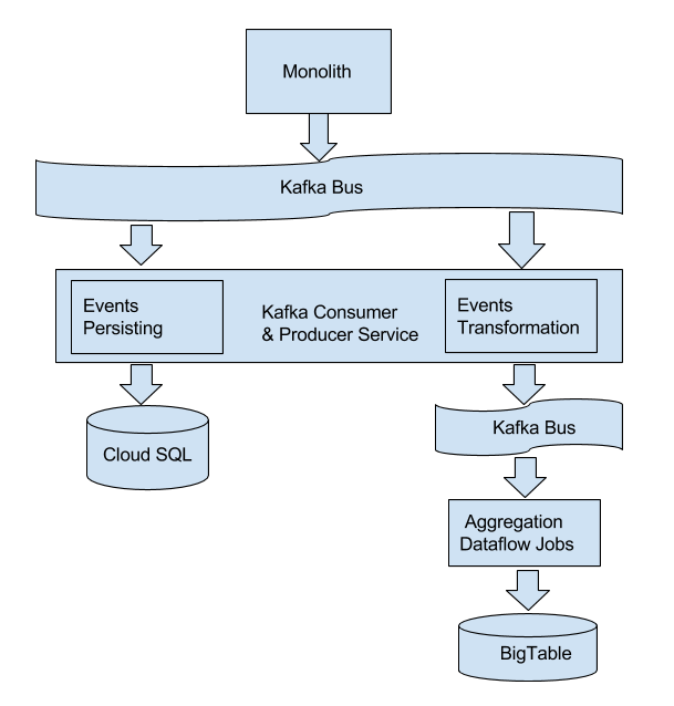
Figure 1. High-level architecture
- The first module is WePay’s monolith service. It publishes Kafka events to a Kafka message bus. Those events are triggered by different checkpoints, and can be categorized into two sets. One category of Kafka events contains static facts information about one entity. For example, the event emitted from user creation actions includes user entity information such as user name, user email, user creation time, and so on. The other category of Kafka events includes some metrics that are aggregated by Dataflow jobs, such as the amount of a payment. Because payment events contain the amount of money for each payment, the total amount of money across all payments for one merchant can be aggregated from Kafka events.
- The second module is a Kafka consumer and producer service that consumes the events published from monolith. It does two kinds of work. For events containing static fact information, the second module extracts transactional information and persists that information into Google CloudSQL, which serves as risk specific storage. For events containing aggregatable metrics, the second module does a series of transformation operations to prepare them for Dataflow ingestion.
- The third module is a collection of Google Cloud Dataflow jobs that poll and aggregate Kafka events published by the second module in both streaming and batch mode. Eventually the aggregation results are persisted into BigTable. For more details on our Dataflow implementation, check out: How WePay uses stream analytics for real-time fraud detection using GCP and Apache Kafka.
Implementation of backfilling
High-level architecture
Fortunately, WePay has a data warehouse built on Google Cloud BigQuery (please see Building WePay’s data warehouse using BigQuery
and Airflow and Streaming databases in real-time with MySQL, Debezium, and Kafka). With that in mind, the method behind backfilling is straightforward:
pulling historical data from BigQuery and pushing it back to our existing pipeline. The solution is described in the diagram below:
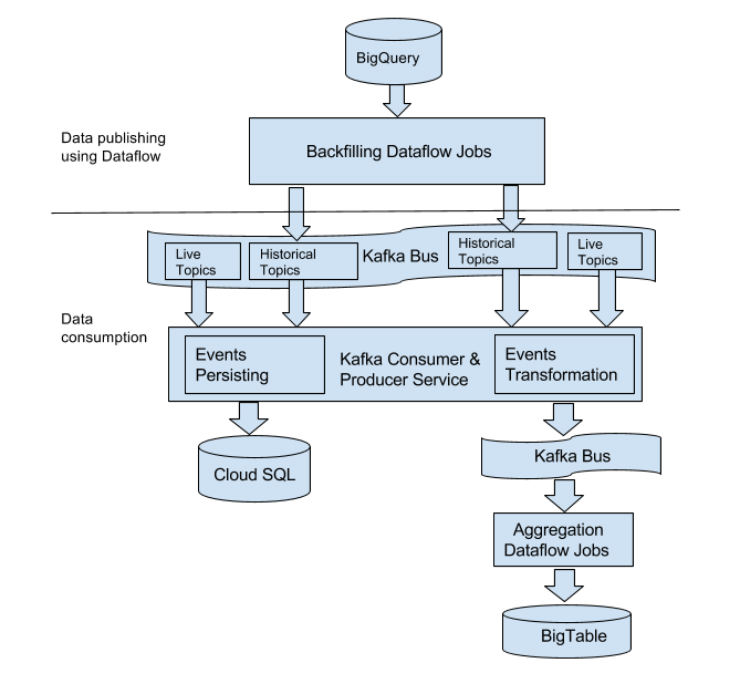
Figure 2. High-level architecture with backfilling
Most parts are the same as our live stream pipeline because we want to reuse our existing functionalities as much as possible. In general, our backfilling mechanism has two sections: data publishing using Dataflow (top part of the diagram) and data consumption (bottom part of the diagram).
Data publishing using Dataflow
A Dataflow batch job is used to pull necessary historical data we need from the data warehouse (Google Cloud BigQuery), and we publish it through the Kafka bus. There are three reasons we chose Dataflow:
- Elastic resource allocation to handle huge batch volume pattern.
- Convenient BigQueryIO SDK that allows Dataflow to consume rows from BigQuery.
- Reusable utilities which can be shared from existing batch and stream Dataflow jobs.
In Figure 2, two kinds of topics are present: “live topics” and “historical topics.” For the live stream pipeline, the monolith publishes Kafka events to Kafka “live topics.” Correspondingly, the backfilling Dataflow jobs query historical data from BigQuery, and publish the same sets of events to the “historical topics.” This isolation of topics ensures that backfilling traffic will not affect our normal live traffic within the Kafka bus. Later, the backfilled Kafka events are aggregated by downstream aggregation Dataflow jobs.
Kafka does provide a log compaction feature that makes it possible to store primary data in Kafka itself, rather than using an upstream store as the primary source of data. One might wonder why we don’t just store all data in Kafka log compacted topics? The answer is practicality and convenience. Kafka is a relatively new piece of infrastructure in our ecosystem, and does not currently have all of the data we need. While we could bootstrap the data into Kafka, and then load it from there, we already have the data in BigQuery. Dataflow makes it fairly easy to push the data where we need it.
Data consumption
The bottom part of Figure 2 represents data consumption, which uses the same service as the live pipeline uses (the Kafka consumer and producer service). The difference is that the consumers to process live stream events keep polling events all the time, as long as the service is live. But the consumers to process backfilled events are created dynamically by an HTTP request. According to the configuration passed through the HTTP request body, consumers either persist transactional data into CloudSQL, or transform Kafka events and publish them for downstream aggregation operations. Both are the same behaviors as noted before in our live stream pipeline. After committing all offsets for the input Kafka topic, the dynamically created consumers free all occupied resources and kill themselves. This method satisfies the following motivations:
- Data migration to support new microservice architecture.
- Applying aggregation logic from the pipeline to historical data.
But how do we make our overall system more resilient? And how do we correct existing data in CloudSQL using backfilling? One common route is that for every Kafka event schema we designed there is a corresponding “modify time” in the payload. During the process of persisting, if the “modify time” in the incoming events is newer or equal to the existing “modify time” in CloudSQL, the corresponding tuple in the database is overwritten.
Validation
We want to verify that each backfilling actually backfills all expected data. The following aspects are taken into consideration when validating:
- Number of tuples returned by the query that backfilling Dataflow jobs used. The backfilling Dataflow jobs use SQL to query BigQuery through BigQueryIO, and each returned tuple may generate at most one Kafka event. There are two methods to achieve this: one is manually querying and another is adding Aggregator statistics in Dataflow jobs.
- Number of Kafka events published by backfilling jobs. This is ascertained through Aggregator statistics, together with a check of the total number of events in Kafka topic.
- Number of records persisted in CloudSQL. A query can be run to check the number of rows in CloudSQL.
For event transformations, we mostly rely on Grafana metrics.
Conclusion
We’ve already loaded more than one and a half years’ historical entity records using this mechanism. The aggregation results can be generated based on backfilled data, so we don’t have to wait several months for the pipeline to catch up. This standardization on a historical data replay mechanism also paves the way for creating new things out of historical data. When we add new metrics in a new system we can easily replay it on historical data and backfill the gaps.