

Logging Machine Learning Data at WePay
Our Goal
At WePay, we use machine learning models for risk analysis and fraud detection associated with payments. Each model is optimized for different fraud patterns and checkpoints associated with the timeline of the payment. Across all models, there is a need for interpretability and retraining. While there is a system in place for this now, the process is time consuming and lacks accuracy. Our goal is to build the underlying system that improves upon this and simplifies the procedures for model maintenance and development. With model logging, our data scientists will be able to accurately extract and understand the historical data in a seamless, efficient and user-friendly way.
Requirements
Our data model needed to be flexible in such a way that it supported an arbitrary number of columns or dimensions of the feature set. We also needed to ensure that the system in place had no effect on model latencies and scaled with the traffic of our payment requests. Finally, we needed to ensure that the quality of the data was exactly the same as the original payloads that entered the model.
Approach
We have a dedicated microservice that is responsible for constructing a model-agnostic payload to send to all model services. Each model would return back a fraud score of the associated payment request along with interpretable reason code(s).
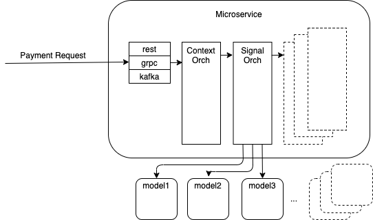
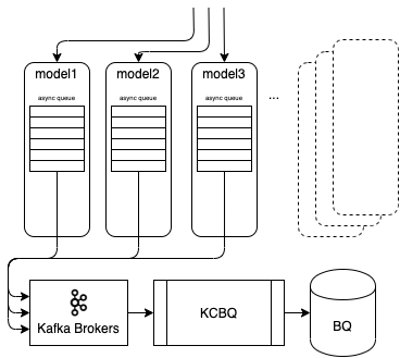
Our approach was to publish Kafka events from each model application to our open sourced implementation of a sink connector from Apache Kafka to Google BigQuery (or KCBQ). We chose Google BigQuery because we already had an infrastructure in place to support it as our cloud data warehouse solution, and it easily scaled with our current volume of requests and expected growth in the future. Additionally, from a business point of view, it allowed our data scientists to query the data in real time to better understand the fraud score surrounding a payment and answer any related questions coming from our risk-analysts.
The payload outbound by the signal orchestrator required a flexible schema for appropriate serialization and deserialization through Kafka and BigQuery. Our schema used Apache Avro with a nested array type data structure in order to accommodate feature vectors of arbitrary dimension.
{
  "type": "record",
  "name": "ModelFeaturesEvent",
  "doc": "Model feature vector or payload.",
  "fields": [
    {
      "name": "modelName",
      "doc": "The name of the model.",
      "type": "string"
    },
    {
      "name": "featureVector",
      "doc": "The list of clean, score-imminent features for the model.",
      "type": {"type": "array", "items": "com.wepay.events.ds.Feature"},
      "default": []
    }
  ]
}
{
  "type": "record",
  "name": "Feature",
  "doc": "A model feature row instance or observation.",
  "fields": [
    {
      "name": "name",
      "doc": "The feature name.",
      "type": "string"
    },
    {
      "name": "value",
      "doc": "The feature value.",
      "type": ["null", "string"],
      "default": null
    },
    {
      "name": "type",
      "doc": "Python-deduced data type of the feature value, necessary for the decoding process.",
      "type": "string"
    }
  ]
}
Using this kind of Avro structure allowed for unnesting to take place within big query as follows:
SELECT
  paymentRequestId,
  (
  SELECT
    f.value
  FROM
    UNNEST(featureVector) AS f
  WHERE
    f.name=singal_id1) AS singalId1
FROM
  `table-name1`
WHERE modelName='model-name1;
Sample output
| Row | paymentRequestId | singalId1 |
|---|---|---|
| 1 | 543123 | 23 |
| 2 | 543124 | 4 |
| 3 | 543125 | 32 |
Road Blocks
A significant problem was the sheer size of individual payloads. Signals entering the models were not always simple numerical data. There were a few instances of type string that were uncapped and scaled in megabytes. This data needed to be transformed and passed through two access points: Kafka and the KCBQ connector. While we could control for the size in Kafka, big query imposed a maximum row size streaming quota of 1MB per row. Whenever a payload’s size exceeded that hard limit, the KCBQ task handling that payload would fail and messages would stop getting logged. Then, because of the frequency of payloads exceeding this size, another task would soon encounter an oversized payload as well and also fail. As this process repeats for all tasks, the connector itself stops.
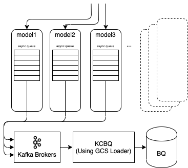
Because signals are added constantly and frequently changing, manually filtering out these signals at the application layer was not a long term solution. Instead, we integrated a new pipeline which first uploads payloads to GCS and then loads them from GCS to BigQuery. The GCS loader is a modification to our KCBQ sink connector which works by changing the way it aggregates rows to write as well as the frequency of upload. It switches from using BigQuery’s streaming API to instead utilizing a batch API for internal load jobs within Google Cloud. The tradeoff it makes is sacrificing the inherent real-time turnaround of streaming each row as it gets produced for the capability of inserting larger amounts of data in a given time window. It also conveniently loosens the limitation of the size of an individual payload. Using our GCS loader, we increased the size constraint to a reasonable scale (100x) or 100MB.
KCBQ’s usual flow uses the BigQuery streaming API to insert data directly as it detects a new record making its way onto the Kafka cluster. Each request to BigQuery comes directly from the connector so the hard limitation of 1MB per row is imposed. When it instead uses the GCS loader it aggregates on N number of rows into a batch before storing them as a JSON file and uploading that as a blob to GCS. It then triggers a load job that loads the contents of this blob to BigQuery. Notably, this load job is internal to Google Cloud which means that the limitation of 1MB per row does not apply. While there is still a limitation of the size of each specific upload using this operation, it is nowhere near as restrictive. An additional consequence of this approach is increased throughput.
Data Verification and Monitoring
Besides relying on the crude metric of logging on the application end, we created custom dashboards with Graphite to validate successful publications to Kafka.
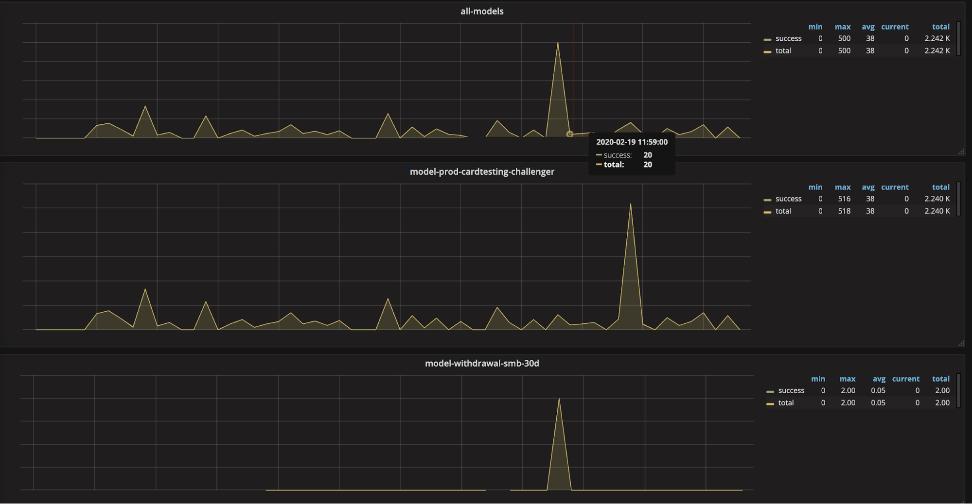
The GCS loader we equipped in our solution is presently in beta, and may have some data consistency issues. To validate against this, we are cross referencing the volume of messages that are successfully logged into Kibana with that into BQ, and examining any particular requests that fall through. In the future, we are planning to put cross-referencing stats in place to report every month on data availability automatically, as well as enable alerting from the graphite dashboards.
End Usage
To wrap this all together, a Python library was written on top of Google’s BigQuery API for the data scientists to use within their own environment and sandboxes (typically Jupyter). A sample query can look like this.
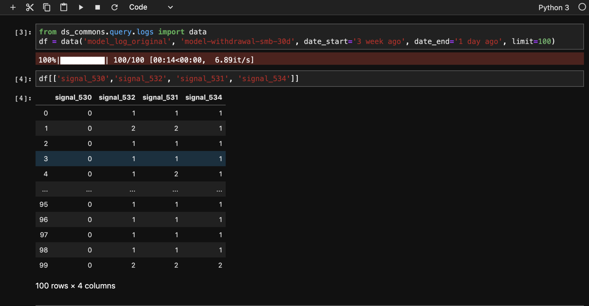
We think this provides the seamless integration we hoped to achieve from the beginning, as well as provide another powerful tool for the data scientists to use. By the way, if you are interested in doing this kind of work, we are hiring!