
BigQuery at WePay
Our previous posts provided an overview of our data warehouse, and discussed how we use Airflow to schedule our ETL pipeline. In this post, we’ll focus on how we’ve set up BigQuery as the database that powers our data warehouse.
Introduction
As we described in our introductory post, WePay used to use a MySQL replica as the place to run analytic queries. This was obviously not a scalable long-term solution. The queries were slow (or timed out), the functionality of MySQL didn’t match with what we needed from a data warehouse, and operating the database became increasingly difficult.
WePay runs on Google Cloud Platform, which includes a solution called BigQuery. BigQuery is a cloud hosted analytics data warehouse built on top of Google’s internal data warehouse system, Dremel. When we began to build out a real data warehouse, we turned to BigQuery as the replacement for MySQL.
BigQuery is an interesting system, and it’s worth reading the whitepaper on the system. It has no indices, and does full table scans for every query. This is a bit counter intuitive. You’d expect such a design to be quite slow. But Google parallelizes the queries, and throws 1000s of machines at the table scans, which speeds up queries pretty dramatically. They are also clever about how they persist data to speed up the full table scans.
Many of the the aggregate queries that never returned in MySQL, or which took more than 24 hours to do so, now take less than a minute in BigQuery. This is not surprising. We weren’t using the right tool for the job. Still, it’s an encouraging outcome that’s worth noting.
The pipeline
Let’s now focus on how we get data into BigQuery. The full flow of data from the source database (a MySQL replica) into BigQuery is as follows:
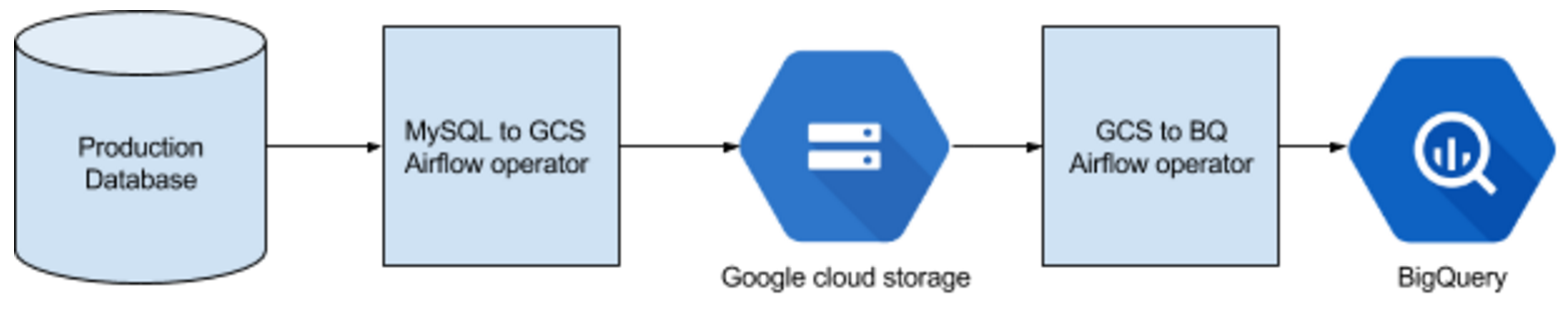
This flow relies heavily on Airflow to orchestrate the data transfers. Airflow’s MySQL to GCS operator is used to load chunks of data from MySQL to Google Cloud Storage. As part of these loads, we also dump the current version of the MySQL table’s schema in a separate JSON file. These two files are used as input in a BigQuery load job, which, again, is an Airflow GCS to BQ operator.
Each table has two main data transfer DAGs. One DAG loads data incrementally every 15 minutes, and a second DAG reloads data every day (at roughly 4 am). The 15 minute pulls happen, unsurprisingly, every 15 minutes. They load the last 30 minutes of data that’s been inserted or updated in each table. The 15 minute overlap (30 minutes of data every 15 minutes) helps in some edge cases, such as delayed MySQL slave replicas, database serializability issues, etc. (documented more in our Airflow post).
The daily 4 a.m. pulls reload data for the entire prior day (overwriting whatever intra-day 15 minute loads happened during that time). This eliminates the duplicate rows that happened during the 15 minute loads, and makes the data in the tables a bit more predictable.
Let’s go through each step in detail.
MySQL to Google Cloud Storage
The MySQL to GCS operator executes a SELECT query against a MySQL table. The SELECT pulls all data greater than (or equal to) the last high watermark. The high watermark is either the primary key of the table (if the table is append-only), or a modification timestamp column (if the table receives updates). Again, the SELECT statement also goes back a bit in time (or rows) to catch potentially dropped rows from the last query (due to the issues mentioned above).
Once the data is selected, it’s loaded into Google Cloud Storage in JSON files. Every execution results in new JSON files. In cases where a data file is larger than two gigabytes, we split the file into multiple chunks to make dealing with the files easier (and BigQuery imposes a four gigabyte per-file limit). The files are stored in a single Google Cloud Storage bucket with the following structure:
json/
  <cluster>/
    <db>/
      <table>/
        dq/
          <YYYYMMDD>/
            <YYYYMMDDHHMMSS>_0.json
        partition/
          15m/
            <YYYYMMDD>/
              <YYYYMMDDHHMMSS>_0.json
          1d/
            <YYYYMMDD>/
              <YYYYMMDD>000000_0.json
schemas/
  <cluster>/
    <db>/
      <table>.json
Our daily DAGs load into the 1d folders for their respective tables and days. Likewise, our fifteen minute incremental DAGs pull data into the 15m table folders. The latest table schema is always stored inside the schemas folder for each table. Note the “_0” for the JSON data files. When we split large table dumps, the counter is incremented for each chunk of the dump.
Note: we also support “full” table snapshots. The Google Cloud Storage structure and behavior is identical to the incremental snapshots, except that no WHERE clause is applied to the select, and every load is a full table over-write (WRITE_TRUNCATE) in BigQuery.
Google Cloud Storage to BigQuery
Immediately after a table’s MySQL to GCS operator is run, a GCS to BQ operator is run to copy the JSON data from Google Cloud Storage into BigQuery. This is a relatively unsophisticated step, since it pretty much just leverages BigQuery’s load job API.
Datasets
The data is loaded into BigQuery datasets according to the format: <cluster>_<db>. For example, if we had a MySQL cluster called ‘fraud’, and a database called ‘models’, then the dataset in BigQuery would be ‘fraud_models’.
Tables
As mentioned above, we have two styles of loading primary database tables into BigQuery: ‘incremental’ and ‘full’. The incremental tables all end with a YYYYMMDD suffix (e.g. model_rankings20160603, model_rankings20160604, etc). BigQuery has built in support for daily table partitioning, and understands this naming scheme. It allows you to use functions like TABLE_DATE_RANGE.
The full table loads are just written with the same table name as their upstream counterpart (no YYYYMMDD suffix).
Note: there is a recently-released new style to table partitioning, which is documented here. We will be moving to this style, and recommend having a look at it.
Handling mutable data
One area that is tricky in BigQuery is how you handle mutable data. BigQuery is append-only, and all writes are treated as immutable–you can’t update a row once it’s been set. This is a great characteristic to have, but we have a seven year old database that includes several iterations of DB schema evolutions. Many of our tables receive updates.
The good news is that (almost) all of our mutable tables have a modify_time field that defines when the row was last modified. Every time the row receives an update, the modify_time is set again. When we do incremental loads on these tables, we use the modify_time to measure our high watermark. But how do we handle the updates in BigQuery?
Every time a row is updated, it gets re-pulled by the latest 15 minute (or daily) snapshot. This means that a row will exist in multiple date partitioned tables, and potentially multiple times within the most recent table. Consider a row that’s been updated on May 3rd, May 29th, and twice on June 3rd. The row would exist in 20160503, 20160529, and twice in 20160603. The most recent row (the one with the most recent modify_time) in 20160603 is the “correct” row now, since it’s the most up to date. This is the row that we want to use. To make this work, we create views for all of our tables. No users ever directly query a table. Instead, they all query views. This allows us to manage permissions in a better way (as we’ll see below), but it also gives us the opportunity to write a deduplication query into our view, so users only see the most recent row.
Here’s an example of a deduplication query for one of our views:
SELECT *
FROM (
    -- Assign an incrementing row number to every duplicate row, descending by the last modify time
    SELECT *, ROW_NUMBER() OVER (PARTITION BY [id] ORDER BY [modify_time] DESC) etl_row_num
    FROM
        -- Get the last month's worth of daily YYYYMMDD tables
        TABLE_DATE_RANGE([project-1234:cluster_db.table],
                         DATE_ADD(USEC_TO_TIMESTAMP(UTC_USEC_TO_MONTH(CURRENT_TIMESTAMP())),
                                                    -1,
                                                    'MONTH'),
                         CURRENT_TIMESTAMP()),
        -- Get all remaining monthly tables prior to a month
        TABLE_QUERY([project-1234:cluster_db.table],
                    "integer(regexp_extract(table_id, r'^table__monthly([0-9]+)'))
                    <
                    DATE_ADD(USEC_TO_TIMESTAMP(UTC_USEC_TO_MONTH(CURRENT_TIMESTAMP())), -1, 'MONTH')") )
-- Grab the most recent row, which will always have a row number equal to 1
WHERE etl_row_num = 1;
This query looks complicated, but it really does something pretty simple. It partitions all rows by their id field (their primary key). It then sorts within each partition according to the modify_time of the row, descending (so the most recent update is first). It then takes only the first row from each partition (the most recent row). This is how we deduplicate all of our tables.
It’s important to point out that this is done at query time. It adds steps to each query, which slows things down a bit, and adds some cost (since data must be scanned more than once). An alternative approach would be to do the deduplication at write time, or some combination of write and read time. Given how frequently we write to tables (every 15 minutes), it’s worked well for us to deduplicate at query time.
Note: the union of the daily and monthly tables is legacy complexity that’s no longer needed. As mentioned above, BigQuery now properly supports YYYYMMDD partitions. Each partition used to be treated as a separate table, and BigQuery limits query unions up to 1000 tables. We had some tables that were more than three years old (more than 1000 partitions), so we rolled our daily tables into monthlies to get around this limit. Again, BigQuery has resolved this issue, and we’ll be moving away from this added complexity.
Direct writes
We also have some services that write directly to BigQuery. This integration exists entirely outside of Airflow and our primary MySQL databases. The services use the BigQuery streaming API to write data directly into BigQuery without Google Cloud Storage or bulk data loads. The service accounts for these services are granted write access to their BigQuery datasets, and write their data in accordingly (usually in YYYYMMDD table partitions). This pattern usually occurs for reporting data that a service wishes to expose for ad hoc analytic queries, but isn’t required at all in our production (web service) environment.
Data quality
One of the biggest problems with data pipelines is not getting data in and out of systems, but doing so reliable, without losing data. One of the nice things about BigQuery’s load job is that it has a maxBadRecords configuration. If set to zero, any malformed rows will result in an error of the job load, and our Airflow DAGs will fail, and alert us. This goes a long way in making sure that all of the data that we get out of MySQL is loaded into BigQuery properly.
We’ve also implemented a few checks to make sure that the data that we get out of MySQL is the right data, and that we haven’t dropped any events, or gotten any malformed rows. These checks run every two hours for nearly every table in BigQuery.
Row count checks
This is a simple row count check that validates that the number of rows in the MySQL table is identical to the number of rows in BigQuery. We include some padding, so rather than checking that the COUNT(*)’s from both databases equal each other, we check that both COUNT(*)’s for all rows older than an hour match each other. This is required because the BigQuery tables are always going to be lagging behind the MySQL tables a little bit, since we do periodic loads (every 15 minutes).
Exact checks
We also do range-based checks that validate that each and every row and column is identical in both BigQuery and MySQL. Every two hours, we pull a chunk of data from MySQL, and load it into BigQuery. We then do an outer join on the table’s primary key between the MySQL data that was loaded and what’s in the main BigQuery table for the same range. A BigQuery Javascript UDF is applied to the joined output, and validates that:
- There are no rows in MySQL that aren’t in BigQuery
- There are no rows in BigQuery that aren’t in MySQL
- Every field for the joined row is identical
The outer join query looks like this:
SELECT
    id,
    error,
FROM
    exact_row_match(
        SELECT
            {cols}
        FROM
            {trusted_dataset_table} mysql
        FULL OUTER JOIN EACH
            {untrusted_dataset_table} bq
        ON
            mysql.{col} = bq.{col}
        WHERE
            mysql.{col} >= {{{{ (ti.xcom_pull('{offset_task_id}', key='offset', include_prior_dates=True) or 0) * {chunk}}}}} AND
            mysql.{col} < {{{{ ((ti.xcom_pull('{offset_task_id}', key='offset', include_prior_dates=True) or 0) + 1) * {chunk}}}}} AND
            bq.{col} >= {{{{ (ti.xcom_pull('{offset_task_id}', key='offset', include_prior_dates=True) or 0) * {chunk}}}}} AND
            bq.{col} < {{{{ ((ti.xcom_pull('{offset_task_id}', key='offset', include_prior_dates=True) or 0) + 1) * {chunk}}}}}
    )
The exact_row_match function is the Javascript UDF that does the validation. If any rows don’t validate, it will emit the primary key ID of the mismatched row, as well as an error message like so:
'`' + field_name + '` does not match between MySQL (val=' + mysql_val + ') and BigQuery (val=' + bq_val + ')'
After the queries run, we use Airflow’s BigQuery check operator to validate that there are no bad rows. If there are, the data quality check fails, and we’re alerted.
Permissions
WePay is a payments company, and we care a lot about security. A surprising number of modern tech companies take a relatively lax approach to securing their data. This is not an option for us, since we deal with financial data. Managing BigQuery permissions was an area that took a while to get right, but we’ve finally converged on a solution that’s working for us now.
Datasets
Our BigQuery tables actually exist in three different datasets:
- The primary dataset (fraud_models)
- The full dataset (fraud_models__views_full)
- The clean dataset (fraud_models__views_clean)
The primary datasets house our partitioned tables (YYYYMMDD) that are dumped directly from MySQL, as well as the monthly rollups that we do (see our note above about this). We don’t typically grant anyone read access to these datasets.
The full datasets include views for every table in the primary dataset. The views do a simple TABLE_DATE_RANGE to union all date partitions into a single queryable view, so that our end-users don’t have to worry about unioning data all of the time. The full datasets remain pretty locked down. We don’t grant a lot of users access to them because some of our data is sensitive, and we want to limit access to it.
The most frequently used datasets are the clean datasets. These datasets contain views for each table, which query the underlying full views. These views filter out PII and other sensitive data, though, so our users aren’t exposed to sensitive information by default.
We never load PCI data into BigQuery. This helps limit the scope of our PCI audits and reduces the security exposure from the end-user perspective.
Group management
We manage access through Google app groups. Users are assigned to groups, and groups are assigned access to the various datasets based on their needs. We never directly manage user to dataset access–we used to do this, but it got unwieldy as the number of users and datasets that we had increased.
Service accounts
All of our services run with their own Google service accounts. This allows us to manage per-service ACLs on each dataset, to limit the scope of each service to only the datasets that they need.
Our Airflow instances also run using Google service accounts (except the local developer Airflow instances, which use OAuth 2). We define a series of Airflow Google Cloud Platform connections (usually, team or product based). Each Airflow connection has its own service account, and again we manage access to datasets on a per-service account basis.
Automation
Managing all of the user, group, and service account management via the Google cloud UI got a bit tedious, so we wrote a script to help us manage group and dataset permissions. The script is a fairly simple Python script that takes in a configuration file, which we keep under source control. The dataset permission file looks like so:
'monolith_products__views_clean': {
      'projectOwners': 'OWNER',
      'foo@developer.gserviceaccount.com': 'WRITER',
      'bar@cloudservices.gserviceaccount.com': 'WRITER',
      'baz@project-1234.iam.gserviceaccount.com': 'WRITER',
      'airflow-connection@project-1234.iam.gserviceaccount.com': 'WRITER',
      'some-google-apps@group.com': 'READER'
},
Group membership permissions are similarly defined:
'some-google-apps@group.com': {
    foo@bar.com': 'MEMBER',
    bar@bar.com': 'MEMBER',
    baz@bar.com': 'MEMBER'
},
Every time we alter the permissions, we commit them to our source control, and trigger the script to execute. The script execution updates the state accordingly, and makes sure that there are no erroneous permissions granted that aren’t defined in the configuration files.
Conclusion
We rolled BigQuery out at the beginning of the year. It’s been working very well for us, overall. The performance gains were a big win, and not having to have an operational team deal with propping the system up all the time has been a really strong plus.